


At Inicio, we manipulate terabytes of geographical data, utilizing both worldwide datasets and detailed regional ones. We process, store, and analyze this data to identify the best possible solar project locations in Europe.
Most of the heavy lifting is handled by a PostGIS database—an industry-standard, battle-tested solution for geospatial data manipulation.
When I started working with PostGIS, I encountered a bunch of hurdles along the way. I quickly realized that I was maintaining a mental list of tricks and patterns that I kept having to use over and over to solve my problems. Even now that I have some experience working with PostGIS, I keep coming back to my list, and reusing these tips. In this post, I’d like to write up some of this knowledge, and describe how we solve these problems and how we make the most out of PostGIS at Inicio.
PostGIS can seem like a complex beast, and geospatial data processing is definitely difficult. You need to handle different geometry types, dimensions, spatial reference systems (SRS), geometry errors, indexes, and much more. Our geospatial engineering team had to develop a deep understanding of how PostGIS deals with geometries to be able to fully optimize our algorithm and enable Inicio to identify all the best solar projects in a country in a matter of hours.
A short primer on geometries and their representations
Before we start, it’s important that you get some understanding of the internal representation of geometries in a GIS system, and what types of geometries you may deal with.
The internal representation of a geometry always boils down to coordinates.
Put in simple terms: A Point is a single coordinate pair. A Line is a list of coordinates. A MultiLine is a list of Line s, a Polygon is a list of coordinates that forms a closed line, a MultiPolygon is a list of Polygons, you see the pattern.
There is an additional complexity that comes with polygons: they can have “holes”, also called internal rings. Internal rings are extra polygons that are part of the main polygon and define internal holes (for example, see the Polygon below).

Dataset
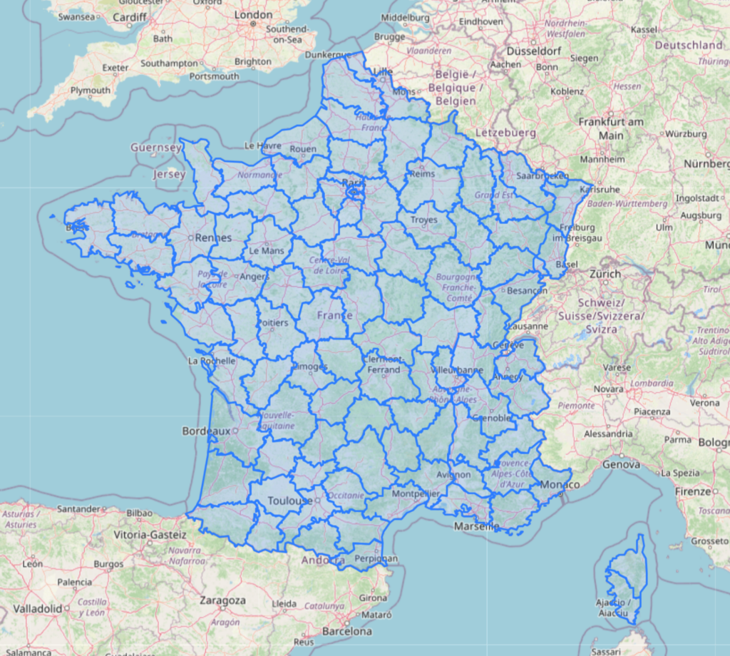
Throughout this post, I’ll use some example geographical data to illustrate the operations I present.
Assume we want to process geometries representing local administrative units. For example, we could be tracking the population density of the country.
ℹ️ Create the dataset yourself
(Measure and) Keep your geometric complexity low
In my opinion, this is the most crucial piece of advice in this article. As a data engineer, you need to know what data you are handling (« what type?« , « how big is it? », « should this relation be represented by foreign key to another table? », « Am I sure this column will fit in a 32bit integer, even as we keep adding rows to the DB?« ).
Similarly, as a GIS data engineer, it’s essential to have a deep understanding of the nature and characteristics of your geospatial data. All of the above applies, but you also need to consider some additional factors specific to geospatial data.
My favorite query to quickly get an understanding of a table’s complexity is the following:
with gis_data_table as (select geometry as geom from department_geoms)
select
    count(*) as num_rows,
    concat(
        round(
            max(st_area(box2d(geom)))::numeric
            / st_area(st_extent(geom))::numeric
            * 100,
            0
        ),
        ' %'
    ) as max_size,
    round(max(st_npoints(geom))::numeric, 0) as max_points,
    round(max(st_nrings(geom))::numeric, 0) as max_rings,
    max(st_numinteriorrings(st_geometryn(geom, 1))) as max_interior_rings,
    concat(
        round((avg((st_area(geom) / st_area(box2d(geom)))))::numeric * 100, 0), ' %'
    ) as squared_geom_metric
from gis_data_table
When we run this query on our department geometries table, we get:
| num_rows | max_size | max_points | max_rings | max_interior_rings | squared_geom_metric |
|---|---|---|---|---|---|
| 96 | 2 % | 582 | 7 | 2 | 55 % |
Let’s briefly go through the columns:
- num_rows: The total number of geometries in the table. So you can get a basic understanding of the dataset size.
- max_size: Is the ratio of the largest geometry’s bounding box area to the total extent of all geometries. This measures how much of the total space is occupied by the largest single geometry. Lower values indicate more evenly distributed geometries.
- max_points: Is the maximum number of points in any single geometry. This gives an upper bound on how detailed or complex your geometries are.
- max_rings: Is the maximum number of rings in any geometry. More rings mean more complex polygons and potentially more processing.
- max_interior_rings: Is the maximum number of interior rings (holes) in the first sub-geometry of each geometry. Similar to
max_rings, more interior rings indicate more complex polygons. - squared_geom_metric: Is the average ratio between the areas of your geometries geometry and their bounding box areas. Higher values indicate more « square-like » or rectangular geometries, which perform better with spatial indexes.
As a rule of thumb for performance critical tables, I try to keep the max_size below 10%, the number of rings and interior rings (max_rings and max_interior_rings) below 100, and the maximum number of points (max_points) below 256. The squareness metric should be as high as possible, while satisfying the other conditions.
This is just a rule of thumb, which is based on our experience working with lots of geospatial data at Inicio, but YMMV!
The results in the table are encouraging news about our table! While the maximum number of points is somewhat high due to the high precision of the administrative boundaries, the other metrics are within acceptable ranges.
Lower values for these metrics ensure better utilization of spatial indexes and keep computations manageable. The speed of geometric operations depends on these values, so tracking them is crucial for maintaining optimal performance. Of course, there is always a tradeoff, and you won’t get all these metrics as low as you want without giving up on some other aspects of your data, like the precision or number of rows.
The rest of this article will give you tools and methods to understand these tradeoffs and how to make the right ones.
Understand spatial indexes
Spatial indexes is what makes PostGIS great. Similar to how normal database indexes work, the goal of a spatial index is to accelerate data lookups.
Creating a spatial index on your table is as simple as writing:
create index gis_index on department_geoms using gist(geometry);
PostGIS spatial indexes are clever things. They are based on an algorithm called R-tree. It works by grouping geometries together based on their bounding boxes in a recursive manner to build a spatial tree of bounding boxes. The leaves of that tree are the geometries.
For more information about how this algorithm works, see the original research paper introducing R-trees. Also this blog post gives a good description of how it works.

Checking that two bounding boxes intersect amounts to doing 4 value comparisons, which can be done on millions of rows in a heartbeat! Using this hierarchical organisation of geometries from their bounding boxes, PostGIS can super quickly narrow down a search to a few geometries by only doing bounding box operations. This often results in a tremendous speedup compared to sequentially scanning your table and checking every intersection.
This means one important thing:
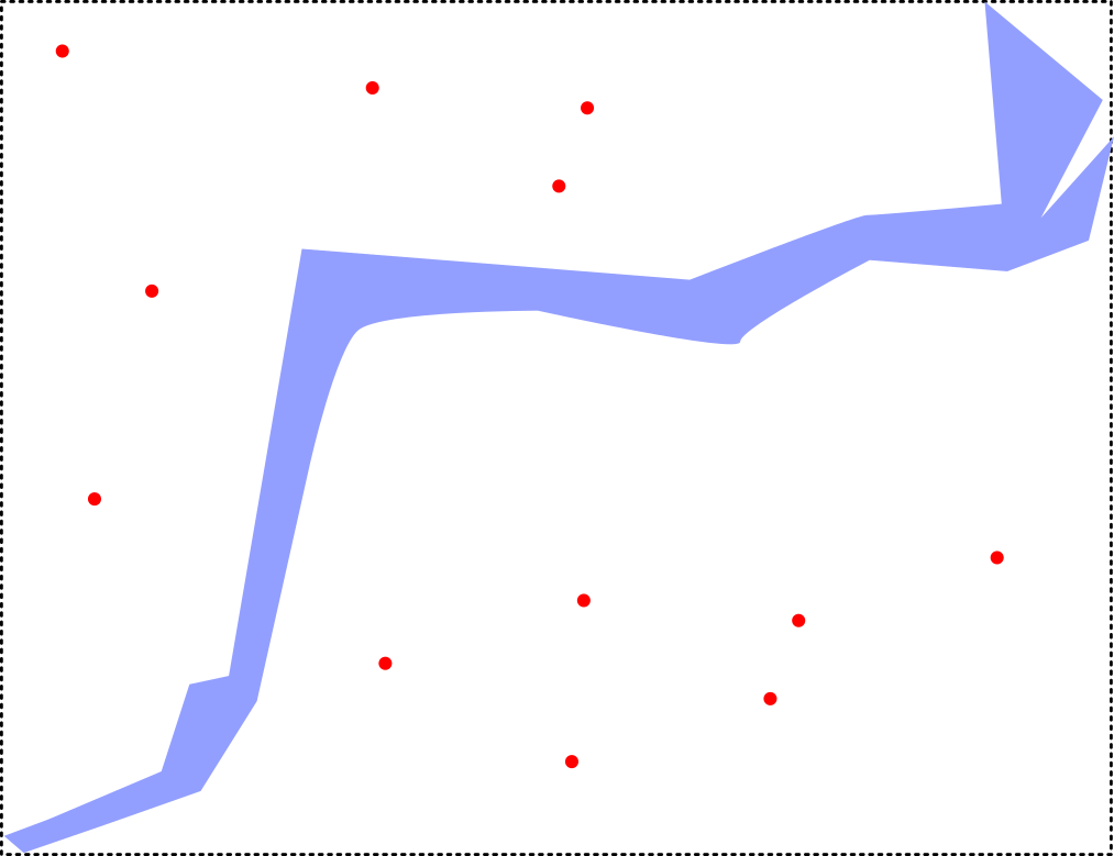
The closer your geometry is to a box (a rectangular geometry), the closer the operation you will be doing is to a simple index lookup. Therefore, the closest you are to a box, the faster the operation will be. Very long and narrow geometries can have a very large bounding box that will result in the index matching many objects that are actually far away from them. This is why it’s important to keep squared_geom_metric high in the complexity metric above.
Let’s visualize this with a simple intersection query. We have randomly generated geometries of different sizes spread out over the country. Let’s call this new table geometry_table.
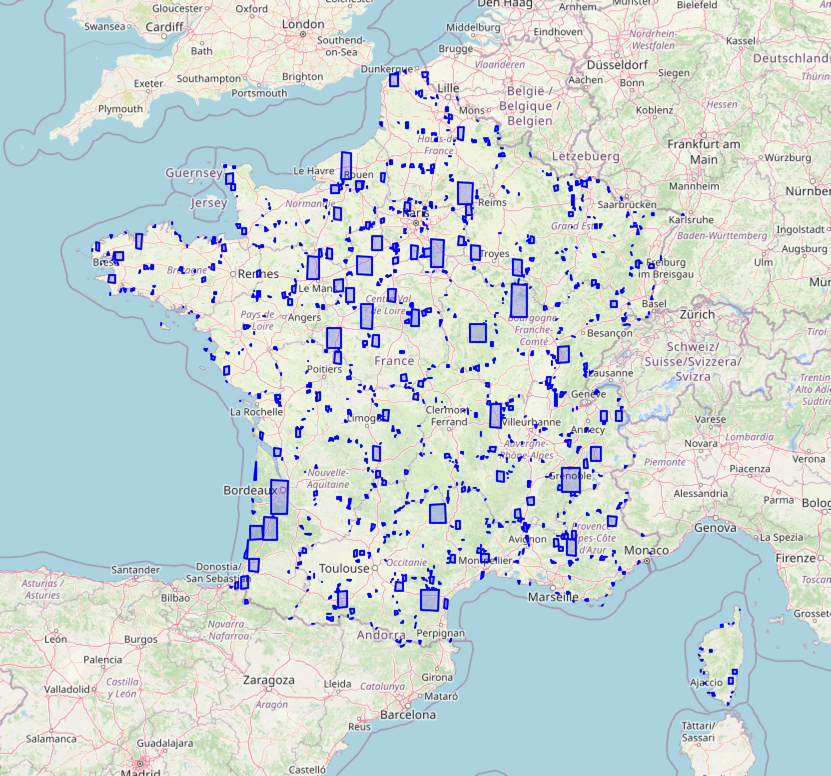
We would like to know the department number of each geometry in geometry_table. For this, we will need to join both tables using an intersection condition.
select department_geoms.code
from geometry_table
join
    department_geoms
    on st_intersects(department_geoms.geometry, geometry_table.geometry)
Depending on your choice of index, you will get wildly different processing times for this very simple query.
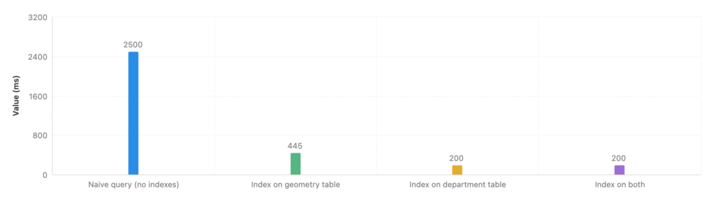
The graph illustrates the significant impact of indexing on a spatial join query performance.
Without indexes, the query takes 2500ms to complete. Adding an index to the geometry table reduces this to 445ms, while indexing only the department table brings it down to 200ms. Interestingly, indexing both tables maintains the 200ms processing time without further improvement.
This show that indexing choices can dramatically improve performance, but additional indexes don’t always provide benefits. In that case, this is because postgres is smart enough to know the department_table index is the best for this query. Understanding your specific data characteristics is always helpful to find the optimal index for geospatial queries.
Subdivide when you work with dense tables
The problem
When doing a lookup in your PostGIS database, indexes are tremendously helpful, allowing you to quickly narrow down your search to a small subsets of objets that are close to the one you care about.
However, for very dense tables, with complex geometries, a spatial index is sometimes not enough. Some issues can also appear if you are comparing geometries of very different scales.
st_subdivide
We have st_subdivide for that! This PostGIS function uses a geometry division algorithm to split geometries into components with less than a certain number of points.
With this function, a single geometry will be converted into several new smaller geometries. If you union them back, you will get the original geometry unchanged. This is an instance of the classic computational complexity vs. storage tradeoff.
Have a look at what happens to our complexity query as we vary the max number of points in our geometries:
Value in
st_subdivide(geometry, {{value}}) |
num_rows | max_size | max_points | max_rings | max_interior _rings | squared_geom _metric |
|---|---|---|---|---|---|---|
| 512 | 125 | 2 % | 508 | 3 | 2 | 54 % |
| 256 | 245 | 1 % | 250 | 3 | 2 | 59 % |
| 64 | 989 | 0 % | 64 | 3 | 2 | 68 % |
| 32 | 2126 | 0 % | 32 | 2 | 1 | 71 % |
| 16 | 3589 | 0 % | 16 | 2 | 1 | 79 % |
By lowering the max number of points, we subdivide more, creating more rows and increasing our “squareness”. This can be very useful to increase the speed of an indexed join operation, since we now know that spatial indexes are better for geometries similar to squares.
When there are too many points, simplify
The problem
Sometimes, you need your geometries to stay more or less the same, and cannot afford to subdivide them because you want them whole. But, if they are still composed of too many points for efficient processing, you’ll need to find a way to make the geometries simpler.
Here comes st_simplify, a PostGIS function that removes vertices from geometries, keeping them the same up to a certain level of tolerance.
st_simplify
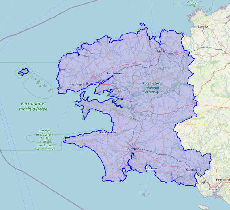
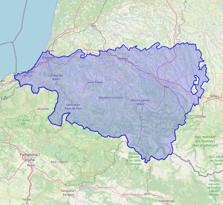
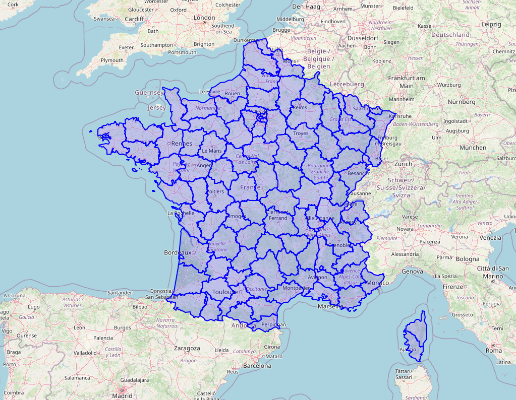
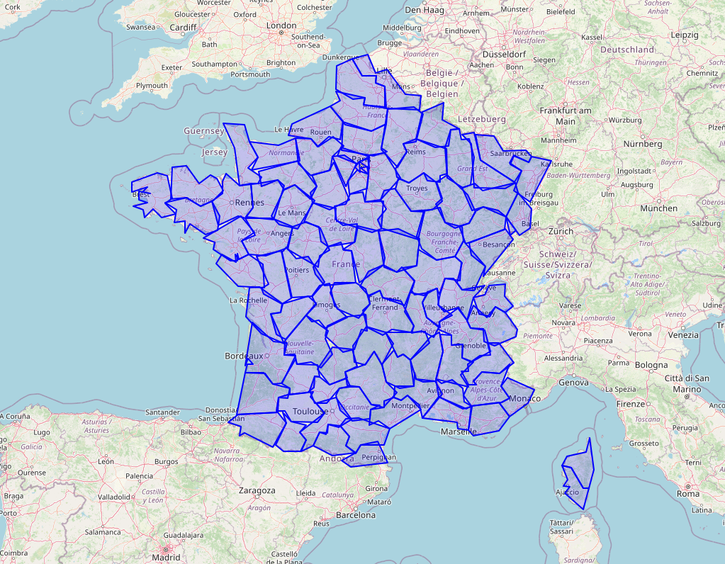
Below, we compare the result of simplification with a tolerance of 1km and a tolerance of 10km. In the first case, we decrease the number of points significantly, while keeping the geometries similar visually (at least from a zoomed out view).
On the other hand, while simplifying with a 10km tolerance brings the max number of points to an extremely low number, it also starts to degrade the shapes a lot.
select
    st_simplify(
        st_transform(geometry, 2154), 1000 -- 1km
    )
from department_geoms
| num_rows | max_size | max_points | max_rings | max_interior_rings | squared_geom_metric |
|---|---|---|---|---|---|
| 96 | 2 % | 179 | 5 | 2 | 45 % |
select
    st_simplify(
        st_transform(geometry, 2154), 10000  -- 10km
    )
from department_geoms
| num_rows | max_size | max_points | max_rings | max_interior_rings | squared_geom_metric |
|---|---|---|---|---|---|
| 96 | 2 % | 19 | 1 | 0 | 43 % |
As you can see, this function allows you to reduce the value of max_points while keeping the values of the other metrics mostly unchanged. We also have no more geometries with « holes » (interior rings).
Learn to deal with various geometries
Inputs are always messy. At Inicio, we deal with hundreds of data sources. Cleaning then up and making sure that the geometries we put in our database are how we expect them to be is crucial.
Here are a few additional functions we use a lot for making sure our geometries are of the right type and that they will behave the way we expect them to.
st_collectionextract
st_collectionextract is a PostGIS function that extracts the geometries of a specific type from a mixed collection of geometries.
For example, if you have Linestring and Polygon in your dataset but only want to « filter » the lines, this is the way to go. It is particularly useful when you have a table with many mixed types resulting from chained operations such as st_intersection, st_union and st_difference. This will create geometries of dimension 0, 1 and 2 (point, lines and polygons), and st_collectionextract can help you get just the ones you need.
See the PostGIS documentation on st_collectionextract for more informations.
st_multi
st_multi is straightforward, and serves a similar purpose as the function above: making sure the geometries are of uniform type. Except that it does the opposite of extracting individual geometries. Points, lines and polygons have a « multi » variant containing collections of these geometries, and st_multi converts input geometries into their multi counterpart.
It can sometimes be useful to ensure you only have « multi » types, especially when you’re exporting data.
st_force2d
This function will ensure your geometry is 2-dimensional, meaning it won’t have an altitude – or z coordinate.
Again, if you are working with external, or user input, this function can act as a filter that ensures all your geometries are homogeneous.
Conclusion
When working with geospatial data in PostGIS, the critical first step is always to understand the complexity of your dataset. Having precise control methods, such as st_simplify or st_subdivide to evaluate and manage this complexity, is extremely valuable. While PostGIS offers many functions and capabilities, establishing this basic understanding of your data’s structure and complexity is essential before applying more sophisticated techniques.
I hope this article will be useful to people working with PostGIS, and will encourage you to explore all the powerful functionalities of this tool for building awesome things with geospatial data.